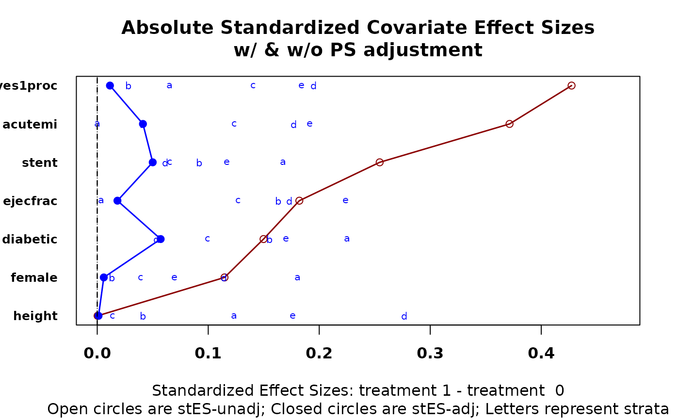
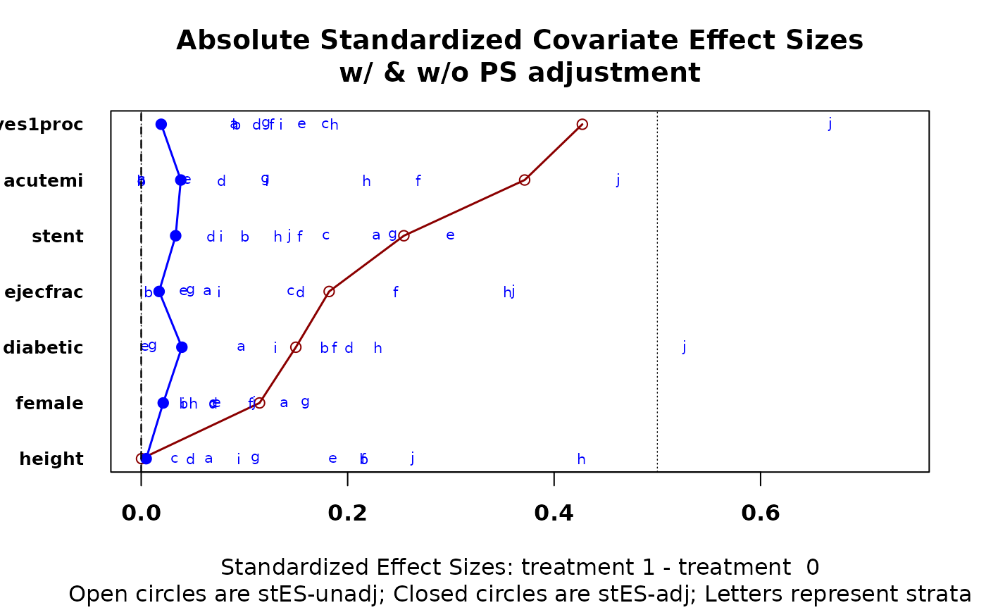
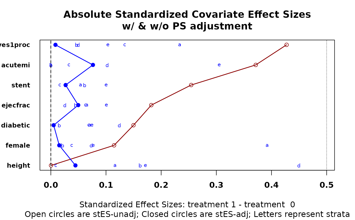
Multiple Covariate Balance Assessment Plot

Provides a graphic that depicts covarite effect size differences between treatment groups both before and after stratification. Function will create stata internally if desired, and returns numerical output used to create graphic.

cv.bal.psa(
  covariates,
  treatment,
  propensity,
  strata = NULL,
  int = NULL,
  tree = FALSE,
  minsize = 2,
  universal.psd = TRUE,
  trM = 0,
  absolute.es = TRUE,
  trt.value = NULL,
  use.trt.var = FALSE,
  verbose = FALSE,
  xlim = NULL,
  plot.strata = TRUE,
  ...
)

Arguments

covariates: Dataframe of covariates. Factors should be recoded using cv.trans.psa
treatment: Binary vector or factor defining the two treatments
propensity: Vector of same length as treatment containing estimated propensity scores.
strata: Either a vector of same length as treatment of predefined stratum number, or one integer n used to assign rows to n strata propensity scores, each of approximately the same number of cases. If relatively few unique propensity scores have been defined (as from a classification tree) then the logical tree should be set equal to TRUE.
int: Either a number m used to divide [0,1] into m equal length subintervals, or a vector containing cut points between 0 and 1 that define subintervals (perhaps as suggested by loess.psa). In either case the subintervals define strata, for which sizes can differ.
tree: Logical, default FALSE. If there are few unique propensity scores, say from a recursively partitioned tree, then TRUE forces strata to be defined by the unique propensity scores.
minsize: Smallest allowable stratum-treatment size. If violated, rows in the stratum are removed. User may wish to redefine strata.
universal.psd: Logical, default = TRUE. Forces standard deviations used to be unadjusted for stratification.
trM: Numeric, default = 0; passed to mean for trimming purposes.
absolute.es: Logical, default TRUE. If TRUE, graphic depicts absolute values of all effect sizes. Note that the adjusted effect size plotted is the absolute value of weighted averages of the signed by-stratum effect size values when absolute.es is TRUE.
trt.value: Character string; if desired allows the name of an active treatment to be given. Should be a level (value) of the treatment factor (vector).
use.trt.var: Logical, default FALSE. If TRUE, uses just active treatment standard deviations for effect size, as per a suggestion of Rubin and Stuart (see reference below).
verbose: Logical, default FALSE. Numerical output is returned invisibly.
xlim: Binary vector passed to plot for overriding default choices. Default NULL.
plot.strata: Logical, default TRUE. Adds effect size values for individual strata to graphic.
...: Other graphical parameters passed to plot.

Value

Graphic plots covariate balance before and after stratication on propensity scores. The default version (absolute.es = TRUE) plots the absolute values of effect sizes for each stratum, though the overall estimate is the weighted mean before taking the absolute values. Numerical output consists of seven addressable objects. If verbose is FALSE (default), output is not printed.

original.strata: Matrix of strata-treatment counts as originally input.
strata.used: Matrix of strata-treatment counts used in effectsize calculations after any minsize reductions.
mean.diff.strata.wtd: Matrix of strata by covariate weighted (by strata size) average differences.
mean.diff.unadj: Matrix of covariate effects sizes before stratification.
effect.sizes: Matrix of effect sizes by covariate and statum.
treatment.levels: Names of treatments.
effects.strata.treatment: Matrix of standard deviations and stratum-treatment covariate means used to calculate the effect.sizes.

Details

Effect sizes between treatments for each covariate are presented in one graphic, both before and after stratification.

References

``Matching Methods for Causal Inference: A review and a look forward." Forthcoming in Statistical Science.

Author

Robert M. Pruzek RMPruzek@yahoo.com

James E. Helmreich James.Helmreich@Marist.edu

KuangNan Xiong harryxkn@yahoo.com

Examples


data(lindner)
attach(lindner)
#> The following objects are masked from lindner (pos = 3):
#> 
#>     abcix, acutemi, cardbill, diabetic, ejecfrac, female, height,
#>     lifepres, stent, ves1proc
#> The following objects are masked from lindner (pos = 4):
#> 
#>     abcix, acutemi, cardbill, diabetic, ejecfrac, female, height,
#>     lifepres, stent, ves1proc
#> The following objects are masked from lindner (pos = 5):
#> 
#>     abcix, acutemi, cardbill, diabetic, ejecfrac, female, height,
#>     lifepres, stent, ves1proc
#> The following objects are masked from lindner (pos = 6):
#> 
#>     abcix, acutemi, cardbill, diabetic, ejecfrac, female, height,
#>     lifepres, stent, ves1proc
lindner.ps <- glm(abcix ~ stent + height + female +
      diabetic + acutemi + ejecfrac + ves1proc,
      data = lindner, family = binomial)
ps<-lindner.ps$fitted
lindner.cv <- lindner[,4:10]
cv.bal.psa(lindner.cv, abcix, ps, strata = 5)

cv.bal.psa(lindner.cv, abcix, ps, strata = 10)

cv.bal.psa(lindner.cv, abcix, ps, int = c(.2, .5, .6, .75, .8))