Clustering Overlap Metric for Determining the Optimal Number of Clusters
Source:vignettes/clustering_overlap_metric.Rmd
clustering_overlap_metric.RmdData preparation…
data(penguins, package = 'palmerpenguins')
cluster_vars <- c('bill_length_mm', 'flipper_length_mm')
penguins <- penguins[complete.cases(penguins[,cluster_vars]),] # Two observations with missing values
Standardize our two clustering variables…
penguins <- penguins |>
    dplyr::mutate(dplyr::across(all_of(cluster_vars), clav::scale_this))
Clearly there are three clusters…
ggplot(penguins, aes(x = bill_length_mm, flipper_length_mm, color = species)) +
    geom_point()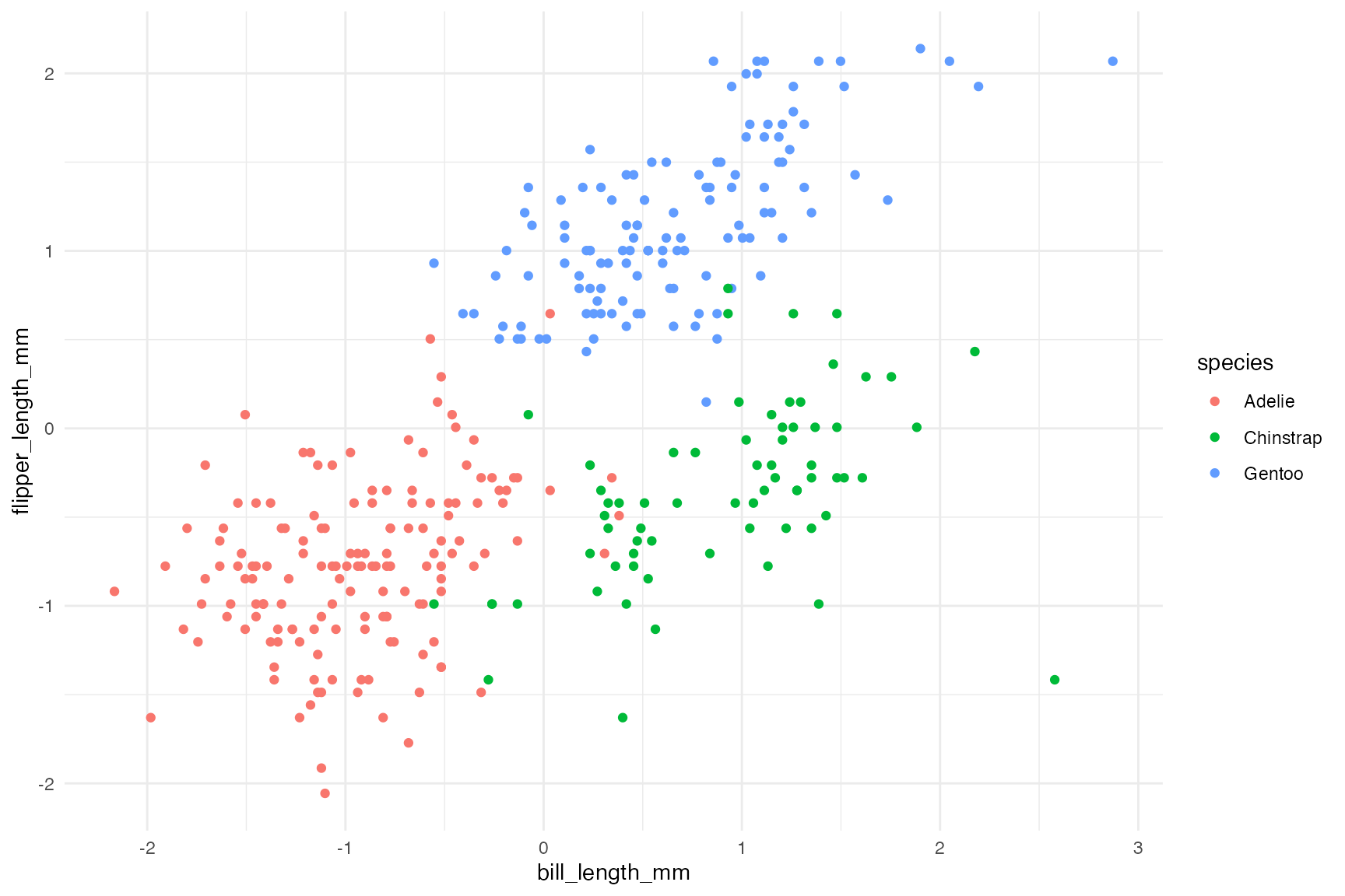
What do some common metrics suggest?
oc <- clav::optimal_clusters(penguins[,cluster_vars], max_k = 6)
plot(oc)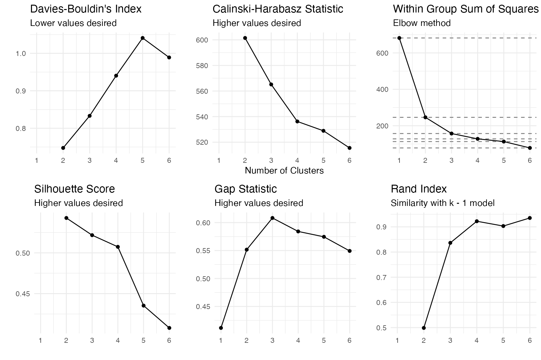
- Davies-Bouldin’s Index: 2
- Calinski-Harabasz Statistic: 2
- Within sum of squares: 3
- Silhouette score: 2
- Gap statistic: 3
- Rand Index: 4
Two of the six metric suggest the actual number of clusters of three.
As describe here the cluster validation uses a bootstrap (or bootstrap like approach) to determine if the clusters are consistent across all the samples. If one of the goals of clustering is for the centers of each cluster to be as far apart from one another as possible, we can use the distributions of cluster means to compare how much they overlap across all bootstrap samples.
Let’s consider the known optimal number of clusters where k = 3.
km_out <- stats::kmeans(penguins[,cluster_vars], centers = 3)
clusters <- km_out$cluster
cv <- clav::cluster_validation(df = penguins[,cluster_vars],
                               n_clusters = 3,
                               sample_size = nrow(penguins),
                               replace = TRUE,
                               verbose = FALSE)
plot(cv)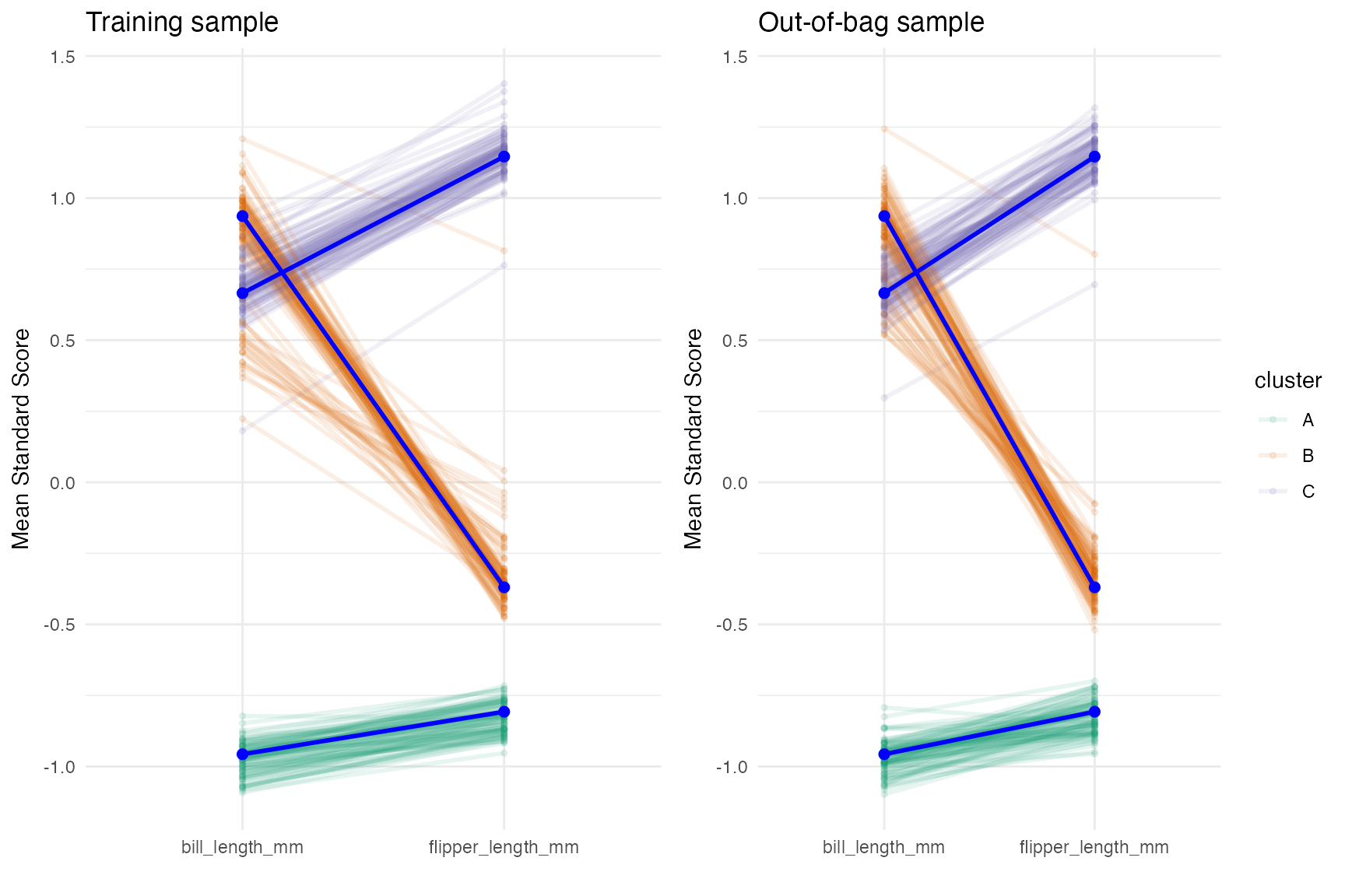
The profile plot above shows that there is pretty good separation,
but the separation between bill_length_mm between clusters
B and C is the smallest. We can see better when we plot the
distributions.
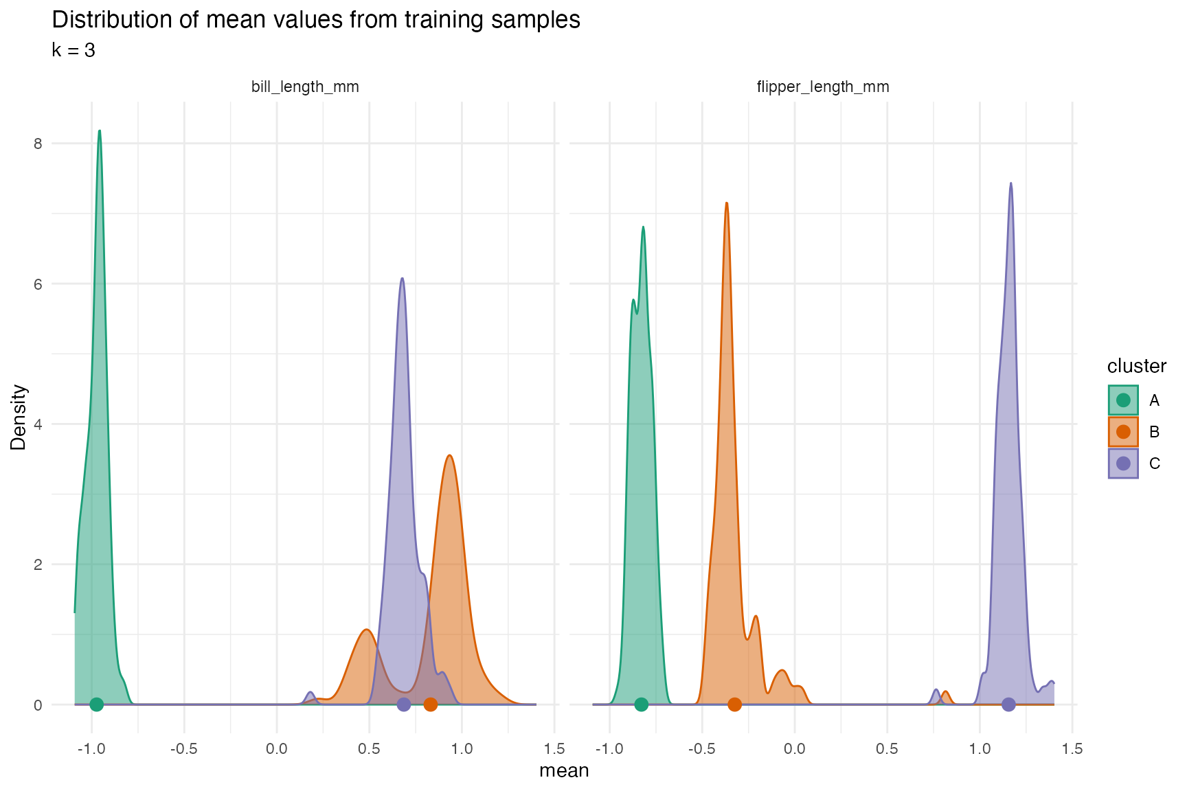
The following table calculates the percent overlap of the distribution of the cluster centers between each cluster for each variable (TODO: that is a wordy sentence).
cv$overlap
#>            variable C1 C2      overlap k
#> 1    bill_length_mm  A  B 7.127233e-17 3
#> 2    bill_length_mm  A  C 5.327061e-17 3
#> 3    bill_length_mm  B  C 1.058899e-01 3
#> 4 flipper_length_mm  A  B 1.202857e-11 3
#> 5 flipper_length_mm  A  C 5.878019e-17 3
#> 6 flipper_length_mm  B  C 9.607188e-04 3
The following function will call cluster_validation and
save the cluster overlap.
#'
#' Note: This will use bootstrapping.
overlap_fits <- function(
        df,
        k = 2:6,
        verbose = interactive(),
        ...
) {
    overlap <- data.frame()
    for(i in k) {
        if(verbose) { message(paste0('Estimating for k = ', i)) }
        cv <- clav::cluster_validation(df = df,
                                       n_clusters = i,
                                       sample_size = nrow(df),
                                       replace = TRUE,
                                       verbose = verbose,
                                       ...)
        overlap <- rbind(overlap, cv$overlap)
    }
    return(overlap)
}
Now let’s try this for k equal to 2 through 6 clusters.
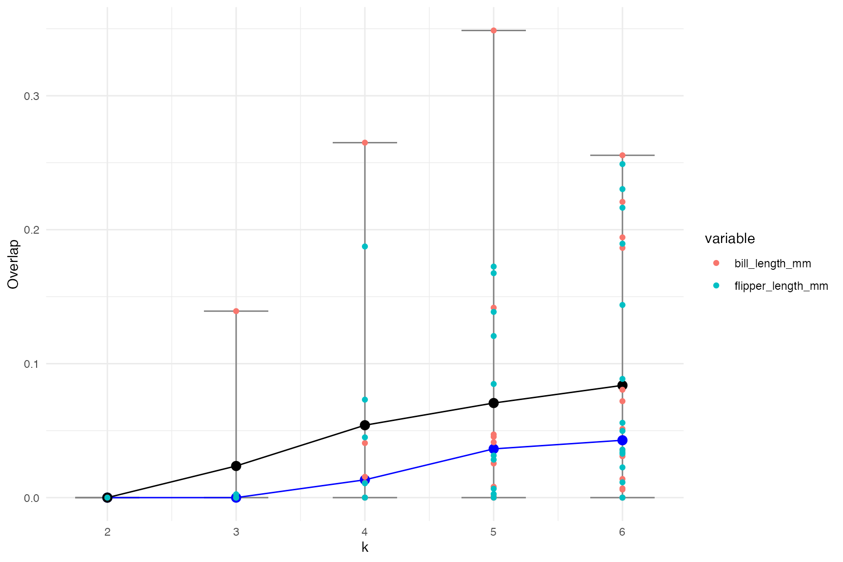
overlap <- overlap_fits(df = penguins[,cluster_vars])The figure below shows the mean (in black) and median (in blue) overlap. The individual points correspond to the overlap for each variable and cluster combination (colored by the variable). Couple of observations from this plot:
- It suggests that k = 3 is the probably the best (well technically 2 but the median difference when k = 3 is the same).
- If there is a large overlap between clusters it is with the
bill_length_mmvariable.
overlap_sum <- overlap |>
    dplyr::group_by(k) |>
    dplyr::summarize(mean_overlap = mean(overlap),
                     median_overlap = median(overlap),
                     min_overlap = min(overlap),
                     max_overlap = max(overlap))
ggplot(overlap_sum, aes(x = k, y = mean_overlap)) +
    geom_errorbar(aes(ymin = min_overlap, ymax = max_overlap), width = 0.5, color = 'grey50') +
    geom_path() +
    geom_path(aes(y = median_overlap), color = 'blue') +
    geom_point(aes(y = median_overlap), color = 'blue', size = 3) +
    geom_point(size = 3) +
    geom_point(data = overlap, aes(x = k, y = overlap, color = variable)) +
    ylab('Overlap')