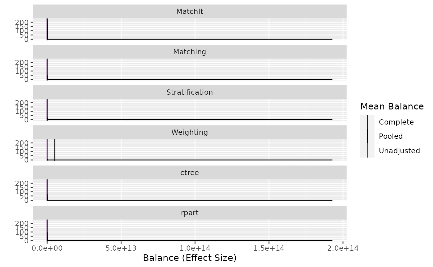
Plot method for balance.

Usage

# S3 method for PSAboot.balance
plot(
  x,
  unadjusted.color = "red",
  complete.color = "blue",
  pooled.color = "black",
  ...
)

Arguments

x: results from balance
unadjusted.color: color of the vertical line representing the mean unadjusted effect size for all covariates.
complete.color: color of the vertical line representing the mean adjusted effect size for all covariates using the complete dataset.
pooled.color: color of the vertical line representing the mean adjusted effect size for all covariates across all bootstrapped samples.
...: currently unused.

Value

a ggplot2 expression.

Examples

# \donttest{
library(PSAboot)
data(pisa.psa.cols)
data(pisausa)
bm.usa <- PSAboot(Tr = as.integer(pisausa$PUBPRIV) - 1,
    Y = pisausa$Math,
    X = pisausa[,pisa.psa.cols],
    control.ratio = 5, M = 100, seed = 2112)
#> 100 bootstrap samples using 6 methods.
#> Bootstrap sample sizes:
#>    Treated=345 (100%) with replacement.
#>    Control=4888 (35%) with replacement.
#> Warning: contrasts dropped from factor ST10Q01 due to missing levels
#> Warning: contrasts dropped from factor ST14Q01 due to missing levels
#> Warning: glm.fit: fitted probabilities numerically 0 or 1 occurred
#> Warning: contrasts dropped from factor ST10Q01 due to missing levels
#> Warning: contrasts dropped from factor ST14Q01 due to missing levels
#> Warning: glm.fit: fitted probabilities numerically 0 or 1 occurred
#> Warning: contrasts dropped from factor ST10Q01 due to missing levels
#> Warning: contrasts dropped from factor ST14Q01 due to missing levels
#> Warning: contrasts dropped from factor ST10Q01 due to missing levels
#> Warning: contrasts dropped from factor ST14Q01 due to missing levels
#> Warning: glm.fit: fitted probabilities numerically 0 or 1 occurred
#> 
bm.usa.bal <- balance(bm.usa)
plot(bm.usa.bal)
#> Warning: Removed 1 rows containing non-finite values (`stat_density()`).

# }